Final Project - Sawyer Force Control

December 15, 2018

Sawyer Force Control

Project Goal

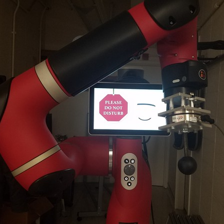
The goal of the final project in my Master’s in Robotics at Northwestern was to implement a force controller on Rethink Robotic’s Sawyer robot. This was to be accomplished using an ATI Axia 80 Force/Torque (F/T) sensor attached to Sawyer’s end effector, in place of its normally attached grippers.

In a very general sense, this project was approached in four steps:

Design and machine adapter plates to rigidly attach the F/T sensor to Sawyer’s wrist
Simulate a motion controller that will be used to drive Sawyer
Adapt the simulated control for use with the real world Sawyer
Use the F/T sensor to control the force applied by Sawyer at the end effector while also controlling Sawyer’s motion

Force control, or being able to control how a wrench is applied at a robots end effector, has many important and impressive uses in industry and research today. For instance, force control can be used to accurately a screw in a threaded hole, or carefully apply a force to a textured surface. In industry, for example, force control can be used to have a robotic arm deburr an arbitrary curved edge. Force control is also used to enhance human-robot interaction by giving the robot the ability to ‘feel’ a human touch and respond in ways that are perceived as natural.

If you are interested in learning more about the ROS package I made for this project, including how to use the package yourself, please see the extremely detailed README on the packages GitHub repository

Please note that the concepts portion of this page much lower down is under construction.

Results

1. Adapter Plates

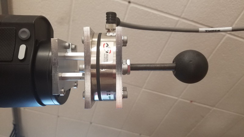
The adapter plates used in this project were designed in OnShape. The design makes use of threaded aluminum spacers to allow access to the screws that attach the plates to Sawyer and the F/T sensor. A plastic spherical knob was threaded on to an M10 threaded rod attached to the bottom adapter plate on the F/T sensor. This allows for smooth contact of surfaces with minimal friction and clean force readings, since the applied force is always perpendicular to the sphere. The full adapter plate and F/T sensor assembly can be seen below attached to Sawyer’s wrist.

ATI Axia 80 Force-Torque sensor attached to Sawyer using custom mounting plates

2. Control Simulator

Running sim_vel_ctrl.launch opens the simulator portion of this package. In this launch file, a trajectory generating node publishes TransformStamped messages representing the desired trajectory along the /desired_trajectory topic. A velocity controller calculates velocity commands to drive the simulated Sawyer’s end effector to this desired transform. These joint positions are then interpolated from these commands and published to be visualized in RViz. The result is a simulated Sawyer following an end effector trajectory described in traj_gen.py, as seen below.

3. Sawyer Velocity Control

After connecting to Sawyer, running sawyer_vel_ctrl.launch begins a velocity control loop that drives Sawyer’s end effector to the trajectory defined in traj_gen.py. Running Sawyer in velocity control mode means its joints can be ran as fast as the internal joint velocity limits will allow. This is very fast. If given a quick trajectory in traj_gen.py Sawyer would happily track this position fast enough to damage something or injure something in the way. Joint velocity commands are limited in sawyer_vel_ctrl.py to 0.6 rad/sec maximum because of this, to prevent accidents. The following gif is a short example of this velocity control running.

A demo of the sawyer_vel_ctrl launch file

4. Sawyer Force Control

After connecting to both Sawyer and the F/T sensor (which also connects over ethernet), running the unidirectional_force_control.launch file will start the packages interaction control capabilities. This launch file attempts to drive the wrench measured by the F/T sensor at the end effector to a desired wrench defined in force_ctrl_traj_gen.py. Unlike traditional hybrid force-motion control, described in detail below, this force control attempts to define trajectories in an attempt to counteract the perceived force error at the end effector. The end effector is driven to these trajectories by the velocity controller. The result represents an approximate force control, as it is not extremely accurate. The following gif show the force controller attempting to maintain a 0 Newton force in the x direction (relative to Sawyer’s base frame). Note how Sawyer attempts to move away from my hand as I try to apply force to the end effector.

A demo of the unidirectional_force_control launch file

Here’s the same launch file running with some more aggressive control gains on both the force and motion proportional controls

A more agressive demo of the unidirectional_force_control launch file

Some Concepts

Task Space Velocity Control

The control nodes implemented in this project are largely based off of Chapter 11 in Modern Robotics by Dr. Kevin Lynch. Specifically, they’re based off the book’s definition of task-space control. Minus the use of quaternions, the code closely mimics the controls described on this page, as described as well in the code comments.

Velocity control in the task-space acts to drive the robot’s end effector to a desired end effector position and rotation by calculating the difference between the current position and the desired position, applying a control law to the calculated error, and sending commands to change the speed of each joint on the robot. To summarize the control law:
Given a current end effector configuration $X( t) \in SE( 3)$ and a desired end effector configuration $X_{d}( t) \in SE( 3)$ , error is calculated as a twist would take the end effector from $X$ to $X_{d}$ in a single unit time, defined as

$$[ X_{e}] =\log\left( X^{-1} X_{d}\right) ;[ X_{e}] \in se( 3)$$

Using this error, we can apply the following control law to calculate our desired body twist that will drive our end effector to the desired position.

$$\ V_{b}( t) =[ Ad_{X^{-1} X_{d}}] V_{d}( t) +K_{p} X_{e}( t) +K_{i} \int X_{e}( t) dt$$

Finally, the commanded joint velocities are calculated using inverse kinematics by multiplying our body twist the inverse of the robot’s psuedojacobian.

$$\dot{\theta } =J^{\dagger }( \theta ) V_{b}$$

These velocities are sent to the robot, then the end effector position is calculated and fed back into the system and the whole process loops like that forever. Of course, if the end effector has reached the desired position, then the commanded joint velocities will all be 0.

Task Space Torque Control

Similar in execution to task space velocity control, this control method takes the robot’s dynamic properties into account. Since torque applied to one joint will effect the movement of the entire robot in real world situations, inertial properties, along with gravity, and Coriolis effect must be taken into account for the most precise controls, of which this project does not make use, but would benefit greatly from.
Torque control begins by measuring the task space error in the end effector configuration as done for velocity control

$$[ X_{e}] =\log\left( X^{-1} X_{d}\right) ;[ X_{e}] \in se( 3)$$

Current task space velocity error can also be measured and used in the derivative portion of this control law

$$V_{e} =[ Ad_{X^{-1} X_{d}}] V_{d} -V$$

The task space dynamics, or the dynamics of the robot are represented in two parts, the first being inertial effects and the second being a combination of gravity and Coriolis effects, as follows

$$F_{b} =\Lambda\left( \theta\right) \dot{V}_{b} +\eta\left( \theta, V_{b}\right)$$

We can calculate each joints torques using the psuedoinverse of the body jacobian, similar to what we did to get joint velocities in velocity controls (this is a good way to visualize how end effector velocities and forces are related to the robot’s joints through the body jacobian)

$$\tau =J^{T}_{b}( \theta) F_{b}$$

Using an approximations of the robot’s dynamic properties, we can wrap a control law around the task space dynamics and multiply that law by the psuedoinverse of the body jacobian to get the torque commands that will be sent to the robot as follows

$$\tau =J^{T}_{b}( \theta ) \left( \tilde{\Lambda }( \theta ) \left(\frac{d}{dt}\left(\left[ Ad_{X^{-1} X_{d}}\right] V_{d}\right) +K_{p} X_{e} +K_{i} \int X_{e}( t) dt+K_{d} V_{e}\right) +\tilde{\eta }( \theta ,V_{b})\right)$$

Force Control or Hybrid Position-Force Control

Force control, the main focus of this project, acts to control the force a robot is applying while also controlling the motion of the robot
Since a robot can not apply a force to free space, a surface is required to implement this control scheme
Each surface or contact scenario, such as running an eraser along a flat chalk board or fitting a peg into a hole, introduces constraints to how the robot may move or apply force, called natural constraints
- For instance, in the chalk board example, the robot would be unable to move its end effector through the board, but must also not move away from the board, or else it would no longer apply a force. This results in a natural constraint of zero velocity perpendicular to the board surface.
Artificial constraints must be added to the force control implementation to reflect the natural constrains in each contact scenario. It is interesting to note that natural position constraints result in artificial force constraints and vice versa
- Referring again to the chalk board example, the natural constraint of zero velocity perpendicular to the board results in an artificial constraint of an applied force also perpendicular to the board. This force can either be constant or a force trajectory (as long as that force is applied towards the board).
To clarify further, please see the following figure from Introduction to Robotics: Mechanics and Control by John J. Craig ( $n_{z}$ in this figure refers to a moment along the $z$ axis)

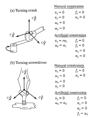
In the first example from the figure above, a robot turning a crank with a spindle handle, the robot is unable to apply velocity into the crank or move up or down relative to the crank, resulting in the natural constraints $v_{x} = 0$ and $v_{z} = 0$ . The robot is also unable to apply rotation along the X or Y axis of the $\{C\}$ (constraint) frame, resulting in rotational velocity constraints at those axises. Similarly, since the crank and handle freely rotate, the robot may not apply a force along the tangential y axis in $\{C\}$ or apply a moment the the spindle along the z axis in the same frame.
- We can see that the chosen artificial constraints reflect these natural constraints. A constant velocity $r \alpha_{1}$ is chosen to be applied in the tangential y axis, resulting in a target rotation speed of $\alpha_{1}$ , as seen in the $\omega_{z}$ artificial constraint.
- Note that these artificial motion constraints correspond to natural force constraints, just as the artificial force constraints of $f_{x}, f_{y}, n_{x}, n_{y} = 0$ correspond to our natural motion constraints
Force control is implemented by applying a motion control scheme (e.g. velocity torque control, as explained above) along directions where artificial constraints specify a motion and a force control scheme along directions where our artificial constraints specify a force (or moment, or both) to be applied.
In this project, as can be seen in the gifs above, Sawyer’s end effector is held in place until a contact force is registered. Then, depending on the set up in the control node, Sawyer will attempt to drive the applied force to 0, effectively avoiding contact, or act against the contact to drive the force along the end effector to a specified value.
This implementation is similar to other hybrid Force-Motion control implementations through its use of Hooke’s Law, where the contact surface is modeled as a spring with a specified stiffness. Adjusting this surface stiffness effectively adjusts the force control loop’s proportional gain.